Visualizing 15-Minute Reachability in the Oslo Public Transit Network

In urban planning and transit analysis, understanding how far residents can travel within a short time frame is a crucial metric. A commonly referenced benchmark is the "15-minute city" concept, where essential services and transit options are accessible within a quarter of a hour. To explore this concept within the context of Oslo, Norway, we generated network visualizations that map the 15-minute reachability between bus stops during the weekday morning peak.

These visualizations highlight the interconnectedness of the city, focusing specifically on the transit service window between 07:00 and 09:00. By evaluating different modes of transportation, we can separate the baseline walkability of the city from the added value provided by the public transit network.

The Foundation: Walking Reachability

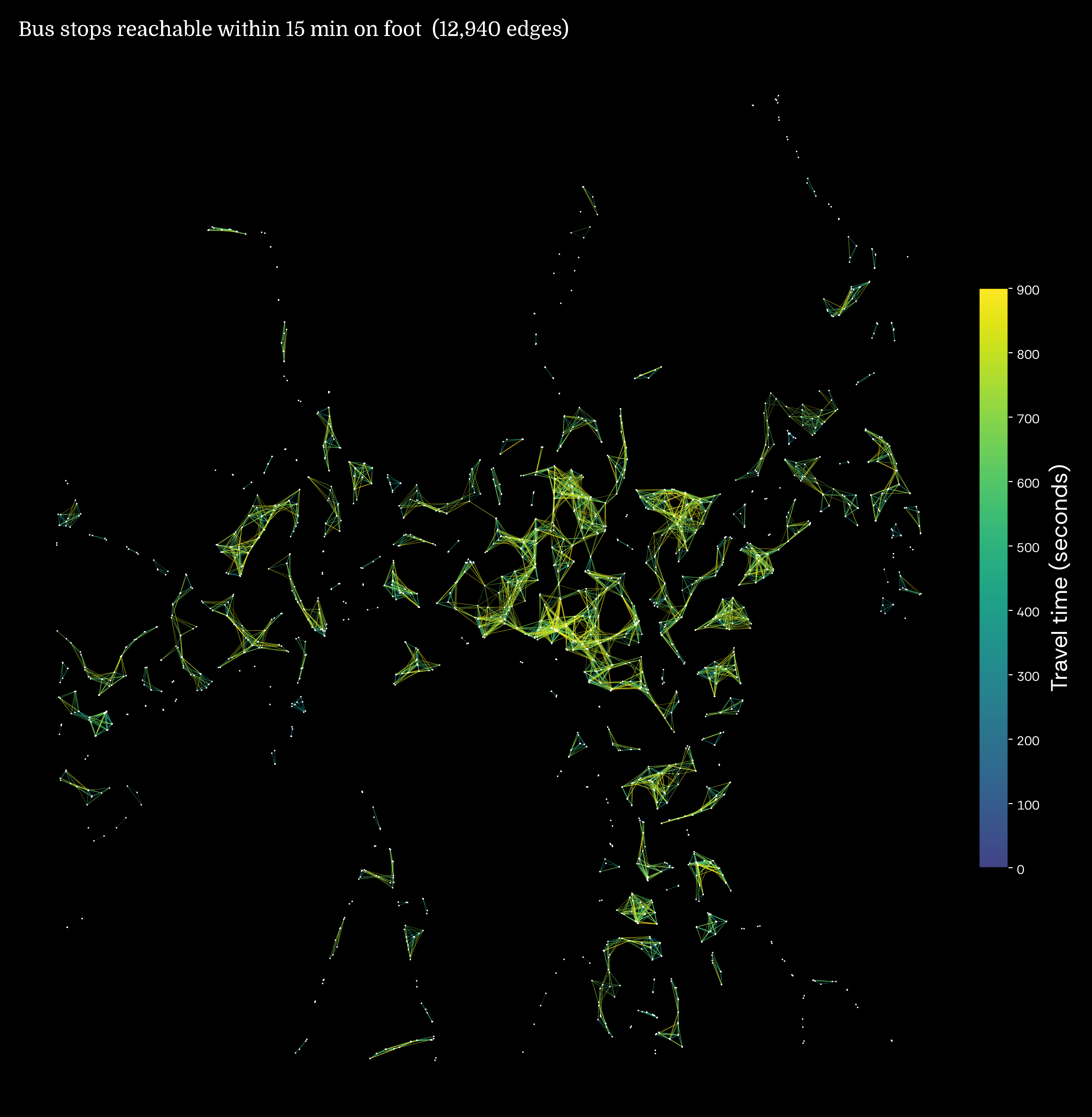
The first visualization maps pairs of bus stops that are reachable within 15 minutes entirely on foot. This serves as our baseline.

This model uses a straight line distance approximation with a standard detour factor to simulate the street network. Assuming an average walking speed of 5 kilometers per hour, the visualization connects neighboring stops to form a dense web of pedestrian accessibility. Because the travel times for walking are distributed evenly across the 15-minute spectrum, the color scale represents the full range from 0 to 15 minutes. The lighter colors indicate shorter walks, while the darker colors approach the 15-minute limit.

This baseline is essential because any journey that can be completed on foot in under 15 minutes is generally more efficient without waiting for a bus.

Walking Reachability

The Transit Advantage: Reachability Requiring Public Transport

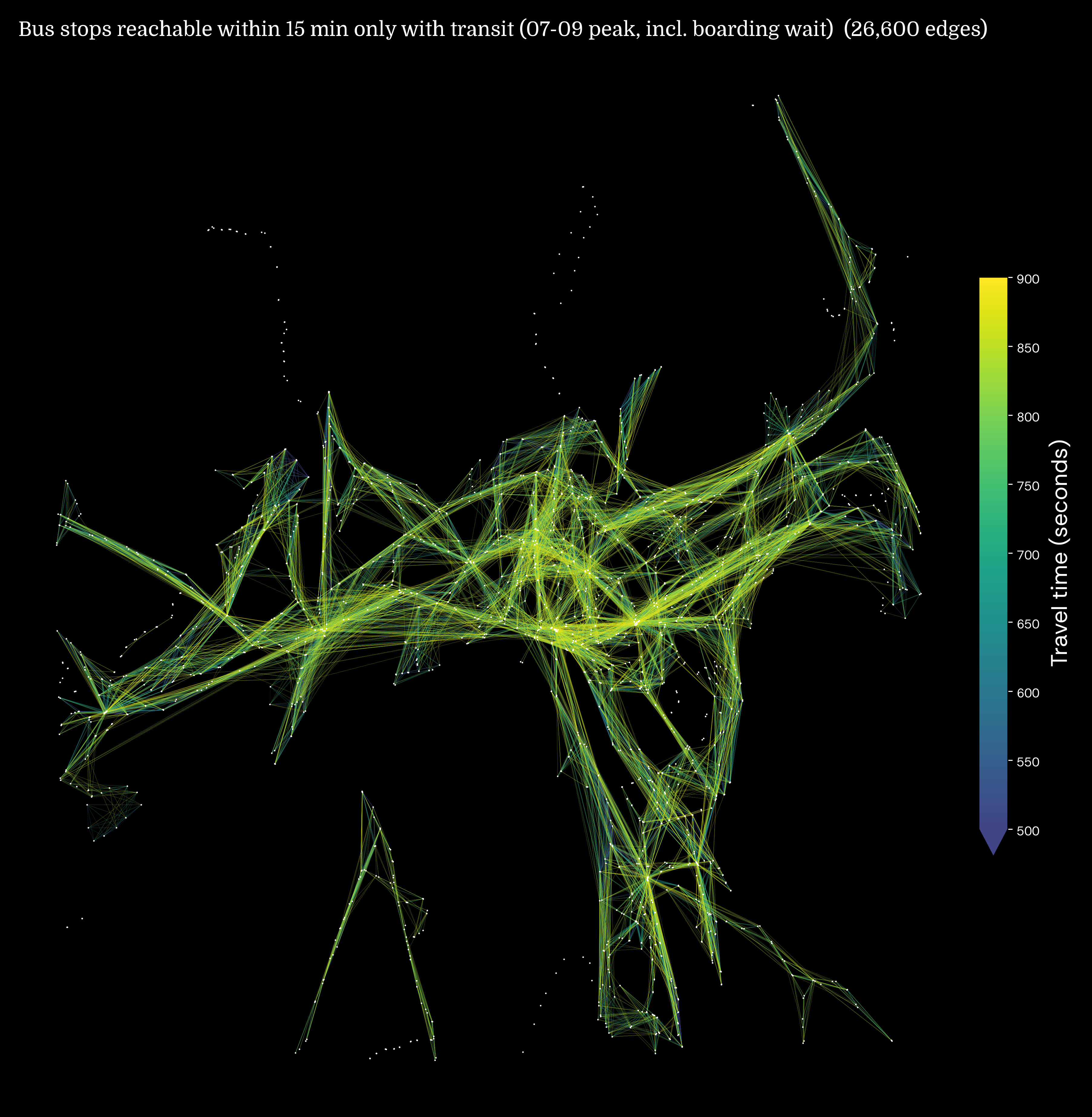
The second visualization demonstrates the specific value added by the transit system. This map displays stop pairs that are reachable within 15 minutes strictly because transit options are available. All stop pairs that could already be reached by walking alone within the same time limit have been removed.

To create an accurate representation of morning peak travel, the transit routing model includes realistic boarding waits. The cost of boarding a vehicle is calculated as half the expected wait time between departures. This means that a direct ride is highly efficient, but transferring between different routes incurs an additional wait time penalty. The routing algorithm considers all local and express bus routes, along with connecting metro, tram, and ferry options.

Because these transit dependent trips often push the boundary of the 15-minute limit, the travel times are heavily clustered near the upper end of the scale. To ensure the map remains legible, the colorbar scale is adjusted to start at the 10th percentile of these travel times. Any trips faster than this threshold are depicted in the lowest color on the spectrum.

Transit Advantage

Visual Design and Interpretation

Both figures are presented on a high contrast black background with white nodes representing the bus stops. The edges connecting the stops are colored according to the travel time required to travel between them. A modified viridis colormap was selected to ensure the figures are colorblind safe, while also maintaining the visibility of shorter, darker edges against the black background.

By contrasting these two maps, we gain a clear perspective on how the Oslo transit network extends the functional range of a commuter beyond simple walking distances. The transit map reveals the specific corridors and connections that make a 15-minute commute possible for a much wider area of the city.

Technical Implementation & Code Reference

This analysis relies on the city2graph library, an excellent tool designed to model urban transit data. The transit data itself is sourced from the GTFS extract for Oslo.

Below, we include the core Python implementation that imports the data, constructs the network, and visualizes the results. These snippets are provided for your reference.

1. Data Import and Configuration

We begin by loading our GTFS data using city2graph and configuring our network boundaries and basic assumptions (such as walking speed and the time window).

Show the code

import warnings
from pathlib import Path
import numpy as np
import pandas as pd
import geopandas as gpd
import matplotlib.pyplot as plt
import matplotlib.cm as cm
import matplotlib.colors as colors
from matplotlib import colormaps
from matplotlib.colors import LinearSegmentedColormap
from scipy.spatial import cKDTree
from shapely.geometry import LineString
import city2graph as c2g

warnings.filterwarnings("ignore", category=UserWarning)
warnings.filterwarnings("ignore", category=FutureWarning)

DATA_DIR = Path("data")
GTFS_OSLO = DATA_DIR / "gtfs" / "oslo_gtfs.zip"   # Oslo-only extract of the Norway feed
FIGURES_DIR = DATA_DIR

CALENDAR_DATE = "20260907"                 # a Monday
OSLO_BBOX = (10.50, 59.80, 10.95, 60.05)   # (min_lon, min_lat, max_lon, max_lat)
METRIC_CRS = "EPSG:25832"                  # UTM 32N, metres
BUS_ROUTE_TYPES = (700, 799)               # GTFS extended route types for buses

WALK_SPEED_MPS = 1.4     # ~5 km/h
DETOUR_FACTOR = 1.3      # straight-line -> street-network distance
WALK_LINK_M = 400        # connect stops within this straight-line distance
THRESHOLD_SEC = 15 * 60  # reachability budget

PEAK_START, PEAK_END = "07:00:00", "09:00:00"   # transit service window
PEAK_WINDOW_SEC = 2 * 60 * 60
MIN_BOARDING_SEC = 60    # floor on the boarding cost
ALIGHT_SEC = 1           # non-zero to preserve edge

gtfs = c2g.load_gtfs(str(GTFS_OSLO))
transit_nodes, transit_edges = c2g.travel_summary_graph(
    gtfs, calendar_start=CALENDAR_DATE, calendar_end=CALENDAR_DATE,
    start_time=PEAK_START, end_time=PEAK_END, directed=True,
)

in_bbox = (
    transit_nodes.geometry.x.between(OSLO_BBOX[0], OSLO_BBOX[2])
    & transit_nodes.geometry.y.between(OSLO_BBOX[1], OSLO_BBOX[3])
)
oslo_stops = transit_nodes[in_bbox].to_crs(METRIC_CRS)
stop_ids = set(oslo_stops.index)

oslo_transit_edges = transit_edges[
    transit_edges.index.get_level_values("from_stop_id").isin(stop_ids)
    & transit_edges.index.get_level_values("to_stop_id").isin(stop_ids)
].copy()
oslo_transit_edges.index.names = ["source", "target"]

2. Network Reachability Calculation

Here we define the walking links and process the route-level transit hops, keeping boarding waits in mind. We then calculate reachability for walking alone versus multimodal transit.

Show the code

def walking_links(src, dst):
    """Walking edges between all distinct (src, dst) pairs within WALK_LINK_M."""
    xy_src = np.c_[src.geometry.x, src.geometry.y]
    xy_dst = np.c_[dst.geometry.x, dst.geometry.y]
    neighbours = cKDTree(xy_src).query_ball_tree(cKDTree(xy_dst), WALK_LINK_M)

    i = np.array([a for a, js in enumerate(neighbours) for b in js if a != b])
    j = np.array([b for a, js in enumerate(neighbours) for b in js if a != b])
    dist = np.hypot(*(xy_src[i] - xy_dst[j]).T)

    return gpd.GeoDataFrame(
        {"distance_m": dist, "travel_time": dist * DETOUR_FACTOR / WALK_SPEED_MPS},
        geometry=[LineString([xy_src[a], xy_dst[b]]) for a, b in zip(i, j)],
        crs=METRIC_CRS,
        index=pd.MultiIndex.from_arrays([src.index[i], dst.index[j]], names=["source", "target"]),
    )

walk_edges = {("transit_stop", "walks_to", "transit_stop"): walking_links(oslo_stops, oslo_stops)}

STOP = "transit_stop"
nodes = {
    "transit_stop": oslo_stops[["geometry"]],
    # route_platforms would be generated from GTFS trip queries (omitted for brevity)
}

def reachability(edges, relation):
    _, out = c2g.add_metapaths_by_weight(
        nodes=nodes, edges=edges, weight="travel_time", threshold=THRESHOLD_SEC,
        new_relation_name=relation, endpoint_type=STOP, directed=True,
    )
    return collapse_directions(out[(STOP, relation, STOP)])

def collapse_directions(edges):
    """One edge per unordered bus-stop pair, keeping the faster direction."""
    u = edges.index.get_level_values(0).to_numpy()
    v = edges.index.get_level_values(1).to_numpy()
    # bus_stop_ids isolates specifically the buses
    keep = (u != v) & np.isin(u, bus_stop_ids) & np.isin(v, bus_stop_ids)
    out = (
        edges.assign(source=np.where(u < v, u, v), target=np.where(u < v, v, u))
        .loc[keep]
        .sort_values("travel_time")
        .drop_duplicates(["source", "target"])
        .set_index(["source", "target"])
    )
    return out[["travel_time", "geometry"]]

def pair_keys(edges):
    return pd.MultiIndex.from_arrays([edges.index.get_level_values(0), edges.index.get_level_values(1)])

# Example generation of walk-only vs transit-assisted reachability
walk_reach = reachability(walk_edges, "15_min_walk")
# transit_with_wait contains combined walk + boarding + ride links 
multi_reach = reachability({**walk_edges, **transit_with_wait}, "15_min_multi_raw")

# We isolate transit-only pairs by removing pairs already reachable by walking
transit_only = multi_reach[~pair_keys(multi_reach).isin(pair_keys(walk_reach))]

3. Plotting the Visualizations

Finally, this snippet generates the high-contrast maps shown above, mapping the calculated travel times to a modified viridis colormap.

Show the code

def truncate(cmap, lo=0.0, hi=1.0, n=256):
    return LinearSegmentedColormap.from_list("trunc", cmap(np.linspace(lo, hi, n)))

BACKGROUND_COLOR = "black"
FIG_SIZE = (12, 12)
SAVE_KW = {"facecolor": "black", "dpi": 300, "bbox_inches": "tight", "pad_inches": 0.2}

# Colour-blind safe; lo=0.2 keeps short edges visible on black
cmap = truncate(colormaps["viridis"], lo=0.2)   

# Transit-only edges cluster near the 15-minute cap, so start their scale at the 10th percentile.
transit_vmin = float(np.floor(transit_only["travel_time"].quantile(0.10) / 100) * 100)

bus_stops = oslo_stops.loc[bus_stop_ids]
minx, miny, maxx, maxy = bus_stops.total_bounds
pad = 0.04 * max(maxx - minx, maxy - miny)
NODE = "bus_stop"

relations = [
    (walk_reach, "15_min_walk", 0.15, "oslo_metapaths_walk.png",
     "Bus stops reachable within 15 min on foot", 0, "neither"),
    (transit_only, "15_min_multi", 0.08, "oslo_metapaths_multi.png",
     "Bus stops reachable within 15 min only with transit", transit_vmin, "min"),
]

for edges, relation, lw, out_name, title, vmin, extend in relations:
    norm = colors.Normalize(vmin=vmin, vmax=THRESHOLD_SEC)
    edge_type = (NODE, relation, NODE)
    edge_colors = list(cmap(norm(edges["travel_time"].to_numpy())))

    fig, ax = plt.subplots(1, 1, figsize=FIG_SIZE, facecolor=BACKGROUND_COLOR, constrained_layout=True)
    ax.set_facecolor(BACKGROUND_COLOR)

    c2g.plot_graph(
        nodes={NODE: bus_stops},
        edges={edge_type: edges},
        ax=ax,
        markersize=1.5,
        edge_linewidth={edge_type: lw},
        node_color="white",
        edge_color={edge_type: edge_colors},
        node_alpha=1,
        edge_alpha=1,
        legend_position=None,
        bgcolor=BACKGROUND_COLOR,
        subplots=False,
    )

    sm = cm.ScalarMappable(cmap=cmap, norm=norm)
    sm.set_array([])
    cbar = fig.colorbar(sm, ax=ax, orientation="vertical", fraction=0.03, pad=0.02, extend=extend)
    cbar.set_label("Travel time (seconds)", color="white", fontsize=18, fontfamily='Rethink Sans')
    cbar.ax.yaxis.set_tick_params(color="white", labelcolor="white")
    for l in cbar.ax.yaxis.get_ticklabels():
        l.set_family('Rethink Sans')

    ax.set_xlim(minx - pad, maxx + pad)
    ax.set_ylim(miny - pad, maxy + pad)
    ax.set_axis_off()
    ax.set_title(f"{title}  ({len(edges):,} edges)", color="white", fontsize=16, loc="left", fontfamily='Domine')

    plt.savefig(FIGURES_DIR / out_name, **SAVE_KW)