Chapter 4 Results
4.1 Model description and tuning
To evaluate different parameter values that are passed to the random forest, a tuning grid needs to be set up. The tuning grid serves the purpose of determining the best combination of parameters according to a range of predefined values for each of those parameters. The ranger implementation was used for this. The mtry parameter, refers to the number of variables that are randomly sampled at each split. In this case the mtry for the tuning grid was defined as mtry=c(2:9). The samp_size parameter specifies the number of samples to train on, spacifying a small number of samples may introduce bias and risk over-fitting. In this case the samp_size was defined as samp_size= c(.65, 0.7, 0.8, 0.9, 1). Finally the node_size parameter defines the complexity of the trees, it determines the minimum number of samples at terminal nodes. For the tuning grid node_size was set as node_size= seq(3,15,by=2). This is shown in the code below:
params <- expand.grid(
mtry= c(2:8),
node_size = seq(3, 15, by = 2), samp_size = c(.65, 0.7, 0.8, 0.9, 1)
)
Once the tuning grid has been defined, a loop that will pass each combination of parameters to the random forest algorithm, saving off the error measure:
for(i in 1:nrow(params)){
rf.i <- ranger(
 formula= reg.mod, data= train_x,
 num.trees= 5000,
 mtry= params$mtry[i], min.node.size= params$node_size[i],
 sample.fraction= params$samp_size[i],
 seed=123
 )
# add OOB error to rf.grid
rf.grid <- c(rf.grid, sqrt(rf.i$prediction.error))
# print to see progress
if (i%%10 == 0) cat(i, "\t")
}
The best performing combination of parameters can be extracted using the which.min function. The best performing combination of parameters is mtry=3, node_size=7, samp_size=0.8, and can be applied to the final model. This is shown in the code below:
rfFit= ranger(
formula = reg.mod,
data=train_x,
num.trees = 5000,
mtry = 3,
min.node.size=7,
sample.fraction =0.8,
seed=123,
importance = "impurity"
)
According to the model, the three most important variables are accommodates, room_type_Private_room, and beds in descending order. This is shown in the figure below:
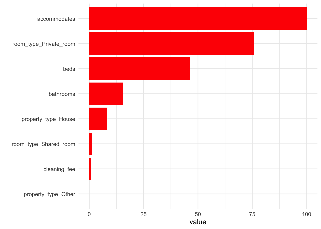
Figure 4.1: Variable importance
4.2 Random Forest Model Results
The Rsquared of the random forest model, is 0.55, suggesting that the final model explains about 55% of the variation. This is shown in the table below, along with the model’s other evaluation metrics.
| RMSE | Rsquared | MAE |
|---|---|---|
| 0.49 | 0.55 | 0.36 |
In contrast, the OLS model’s Rsquared was 0.53, suggesting that the model explains about 53% of the variation. The model specifications are shown below:
reg.mod =
  as.formula(log_price ~ accommodates + beds + bathrooms +
               cleaning_fee + property_type_House +
               property_type_Other + room_type_Private_room +
               room_type_Shared_room)
m = lm(reg.mod, data = data_anal)
summary(m)
##
## Call:
## lm(formula = reg.mod, data = data_anal)
##
## Residuals:
## Min 1Q Median 3Q Max
## -2.0207 -0.3083 -0.0609 0.2217 5.0743
##
## Coefficients:
## Estimate Std. Error t value Pr(>|t|)
## (Intercept) 3.906290 0.025383 153.895 < 2e-16 ***
## accommodates 0.114073 0.005815 19.616 < 2e-16 ***
## beds 0.009721 0.007659 1.269 0.204405
## bathrooms 0.069179 0.013832 5.001 5.89e-07 ***
## cleaning_fee -0.077549 0.016110 -4.814 1.53e-06 ***
## property_type_House -0.163889 0.018433 -8.891 < 2e-16 ***
## property_type_Other 0.069984 0.020292 3.449 0.000568 ***
## room_type_Private_room -0.578816 0.019369 -29.883 < 2e-16 ***
## room_type_Shared_room -0.748410 0.074809 -10.004 < 2e-16 ***
## ---
## Signif. codes: 0 '***' 0.001 '**' 0.01 '*' 0.05 '.' 0.1 ' ' 1
##
## Residual standard error: 0.5183 on 4837 degrees of freedom
## Multiple R-squared: 0.533, Adjusted R-squared: 0.5322
## F-statistic: 689.9 on 8 and 4837 DF, p-value: < 2.2e-16The relative prices predicted by each model for the potential listings provided by the client are shown in the table below:
| ID | OLS.Price | RF.Price |
|---|---|---|
| 1 | $80 | $80 |
| 2 | $40 | $35 |
| 3 | $40 | $35 |
| 4 | $40 | $35 |
| 5 | $110 | $95 |
| 6 | $65 | $70 |
| 7 | $105 | $100 |
| 8 | $30 | $30 |
| 9 | $65 | $70 |
| 10 | $90 | $100 |